计算机视觉的主要任务和进展

计算机视觉任务、可视化和理解

Semantic Segmentation

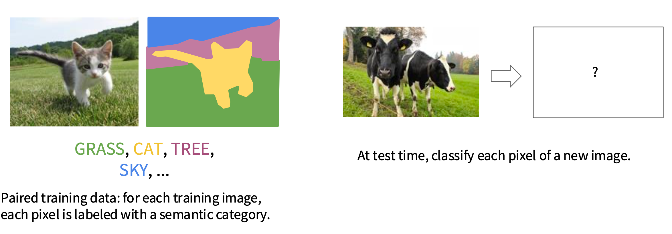
训练集: 给每个像素点 打上语义类别标签

测试 : 给图片的每个像素点分类

思路一: Sliding Window ,上下文提取特征

Learning Hierarchical Features for Scene Labeling(TPAMI 2013)

Recurrent Convolutional Neural Networks for Scene Labeling(ICML 2014)

问题:效率很低,没有利用重叠的patchs的共享features.

思路二:全卷积

idea1: 提取上下文空间特征,不下采样从而保证输出和输入的shape一致$\Rightarrow$ 太贵了

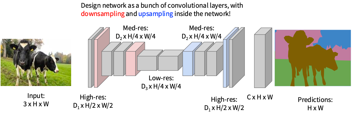
Idea2:先下采样然后再上采样来keep shape

• Fully Convolutional Networks for Semantic Segmentation(CVPR 2015)

• Learning Deconvolution Network for Semantic Segmentation(ICCV 2015)

下采样 : 先Pooling 再 Stride Convolution

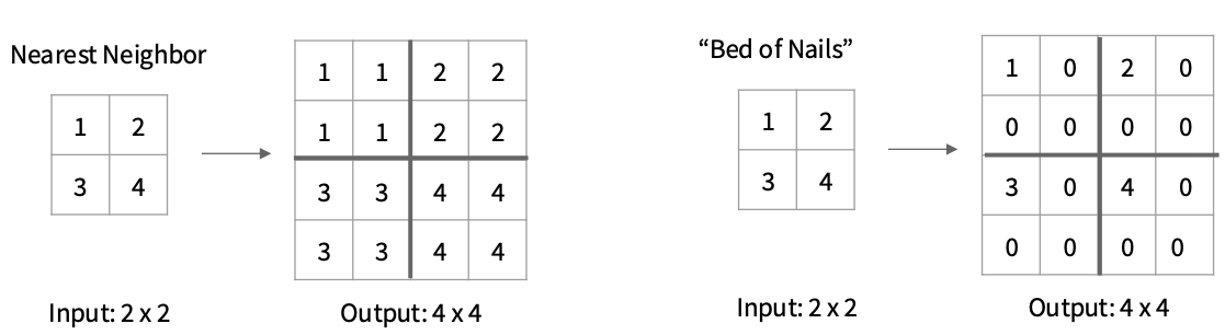
上采样 : Unpooling

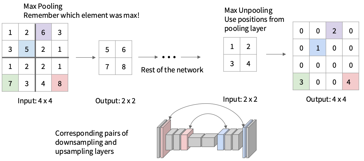
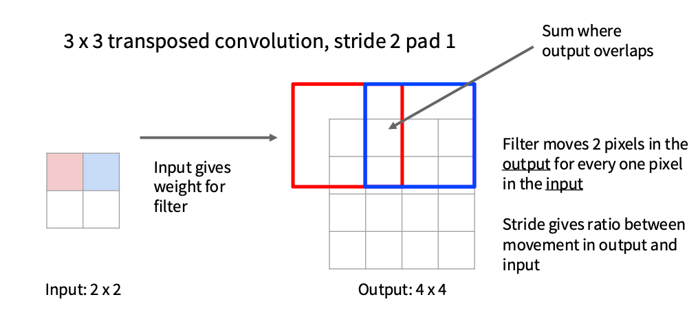
可学习的版本: 反卷积(Transpose Convolution)

思路三: U-Net

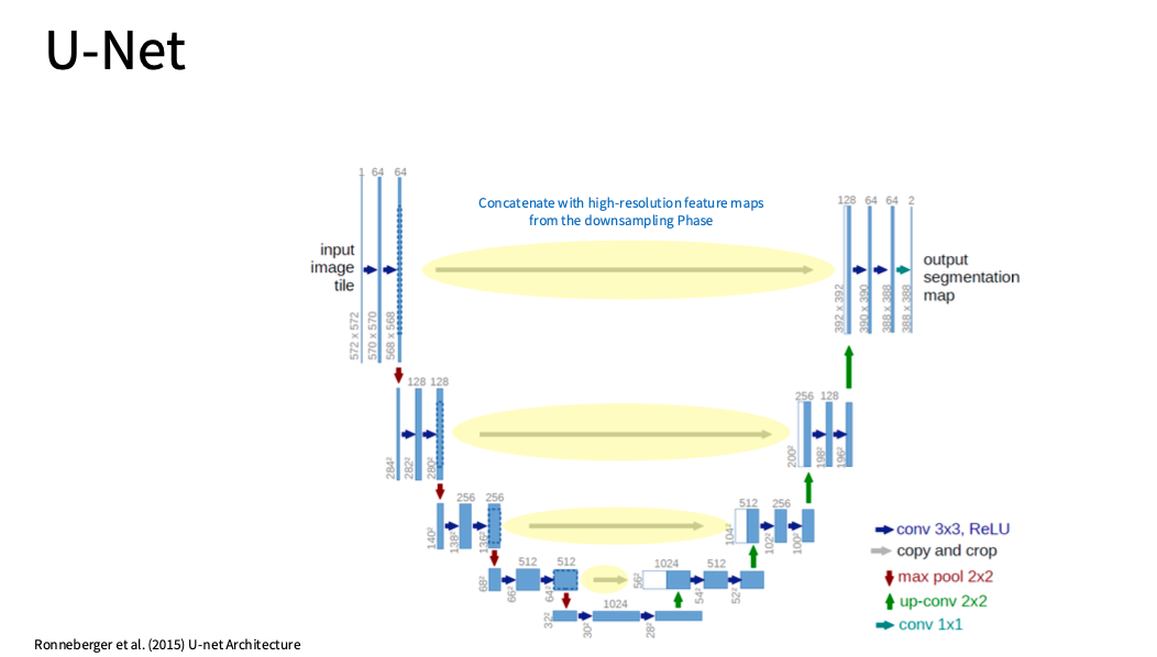
$\color{red} 别关心实例,只关注像素 $​

• 先downsampling 再upsampling

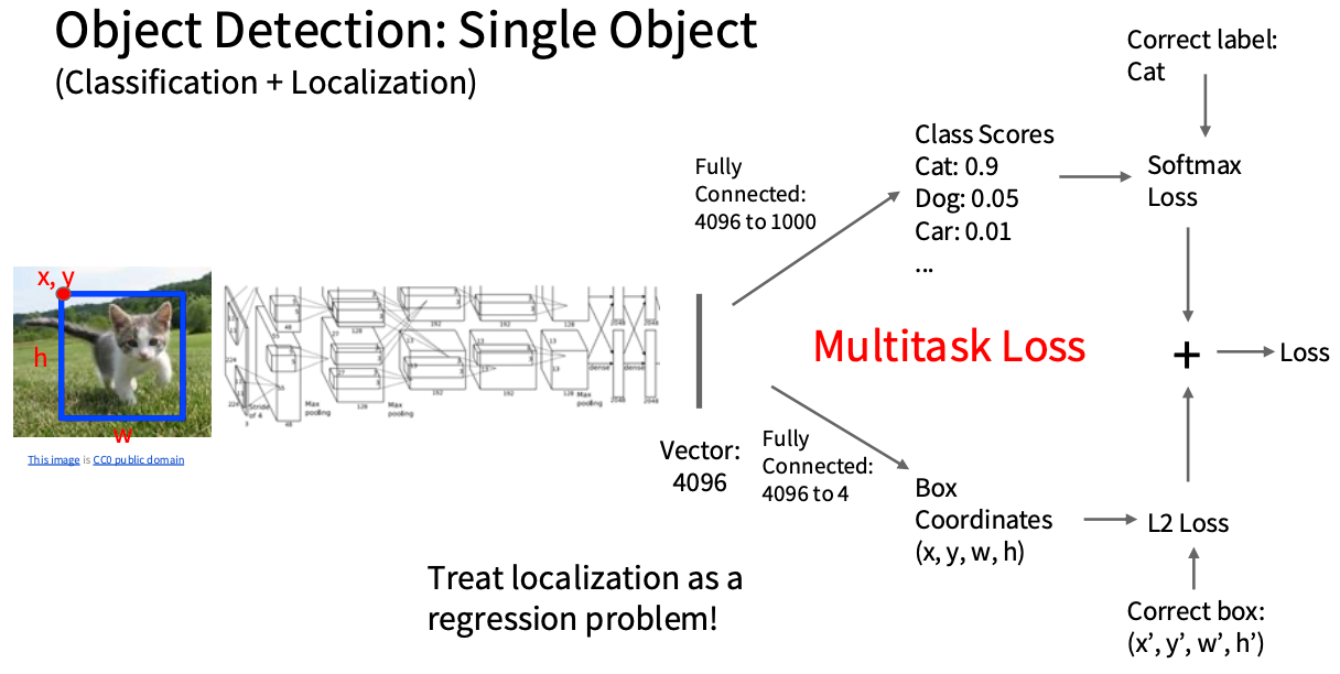
物体检测=Classification + Localization

但是对于多物体检测, Each image needs a different number of outputs!

思路一: 将图片分成多个patch然后分别进行单物体检测

Problem: Need to apply CNN to huge number

of locations, scales, and aspect ratios, very

computationally expensive!

思路二: Region Proposals: Selective Search

● Find “blobby” image regions that are likely to contain objects

● Relatively fast to run; e.g. Selective Search gives 2000 region

proposals in a few seconds on CPU

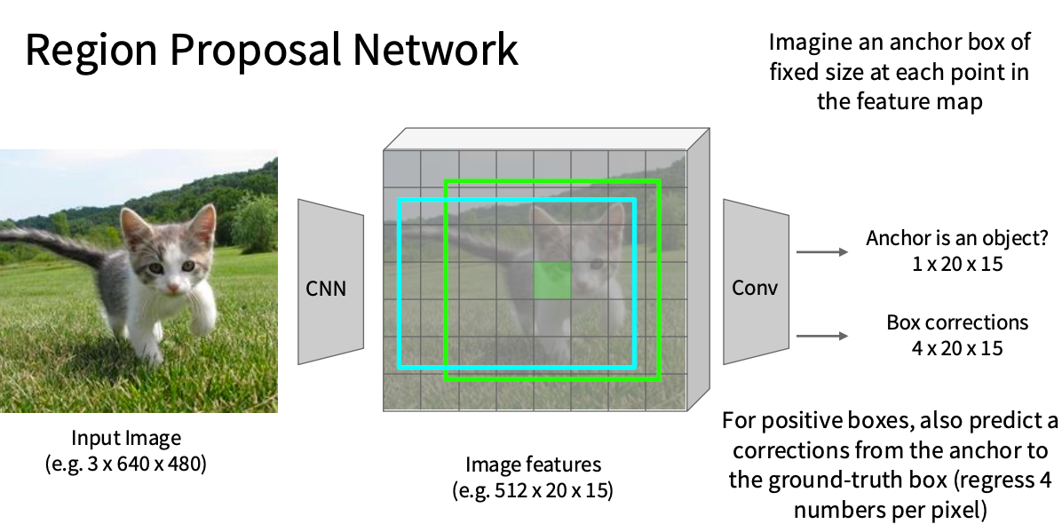
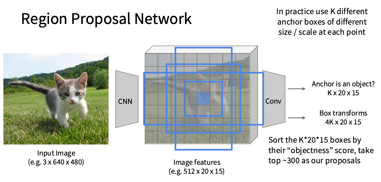
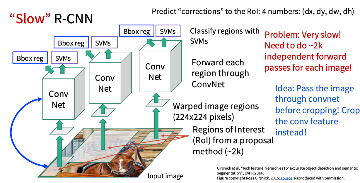
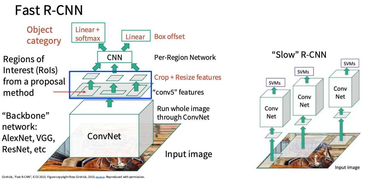
思路三: R-CNN

Rich feature hierarchies for accurate object detection and semantic segmentation(CVPR 2014)

Modern Method

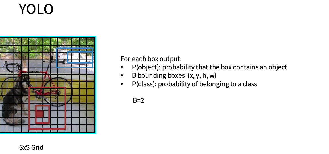
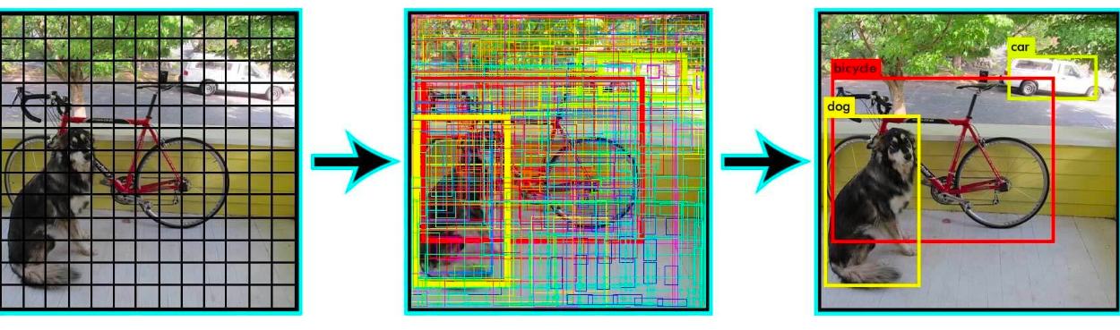
Single-Stage Object Detectors: YOLO / SSD / RetinaNet

Yolo(CVPR 2016)

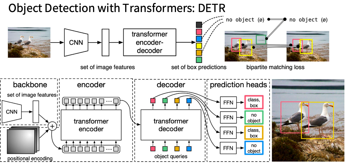
DETR:Object Detection with Transformers(ECCV 2020)

开源框架(Detectron)

可视化(可解释性)

Saliency Maps(ICLR workshop 2014)

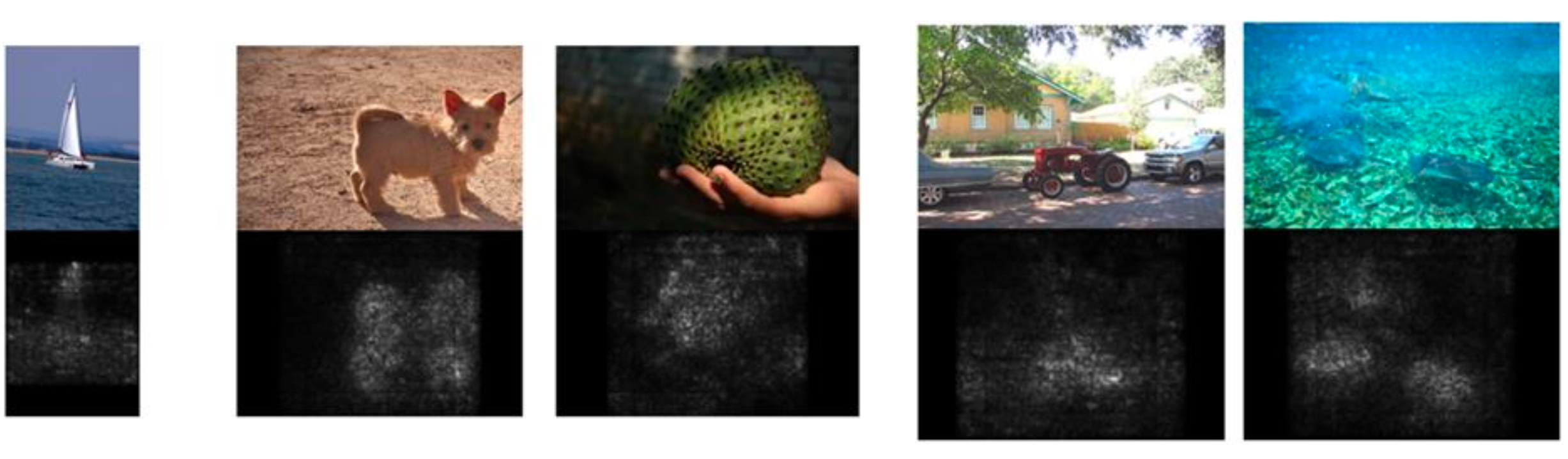
Saliency Maps（显著性图）本质上是：告诉你模型在做某个预测时，“输入的哪些位置/像素最影响这个预测”。通常用一张与输入同尺寸的热力图表示，越亮代表越“重要”。

对某个类别分数 ($S_c(x)$)（比如分类 logits）对输入 (x) 求梯度： \(M = \left|\frac{\partial S_c(x)}{\partial x}\right|\) 直觉：

• 如果某个像素稍微变化，会让类别分数变化很大 ⇒ 该像素对预测很关键 ⇒ map 上更亮。
• 常见做法：对 RGB 三通道取绝对值后再求和/取最大，得到单通道热力图。

优点：简单、一次反传就能算。 缺点：噪声大、容易“看起来很碎”。

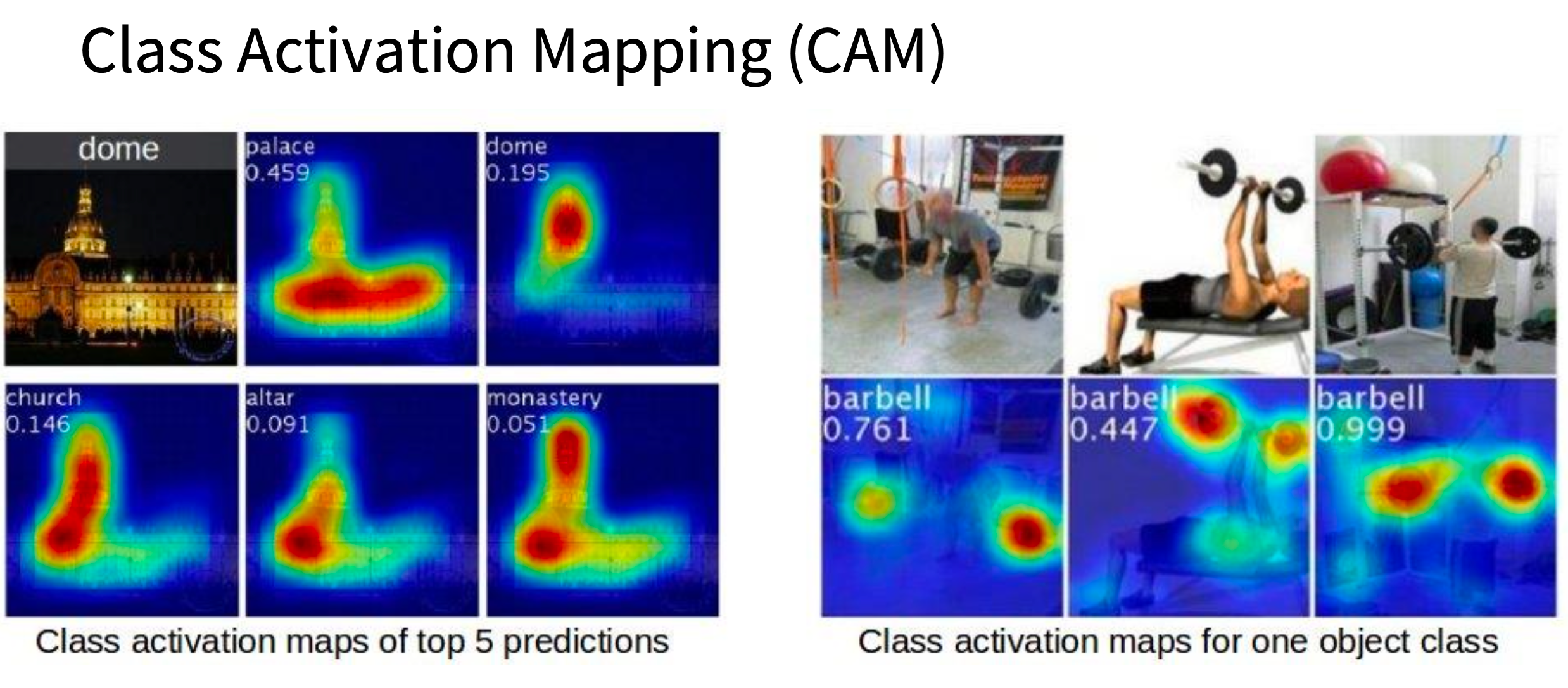
Class Activation Map(CAM)（更像“模型在看哪里”)(CVPR 2016)

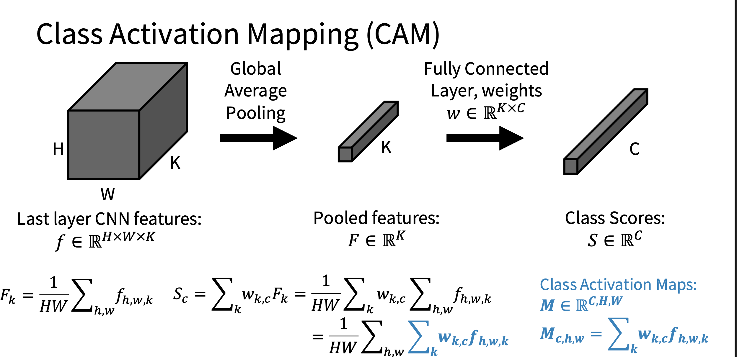
这类不是对输入求梯度，而是用最后一层卷积特征图做可视化。

$\color{red}缺点:只能应用于最后一层$

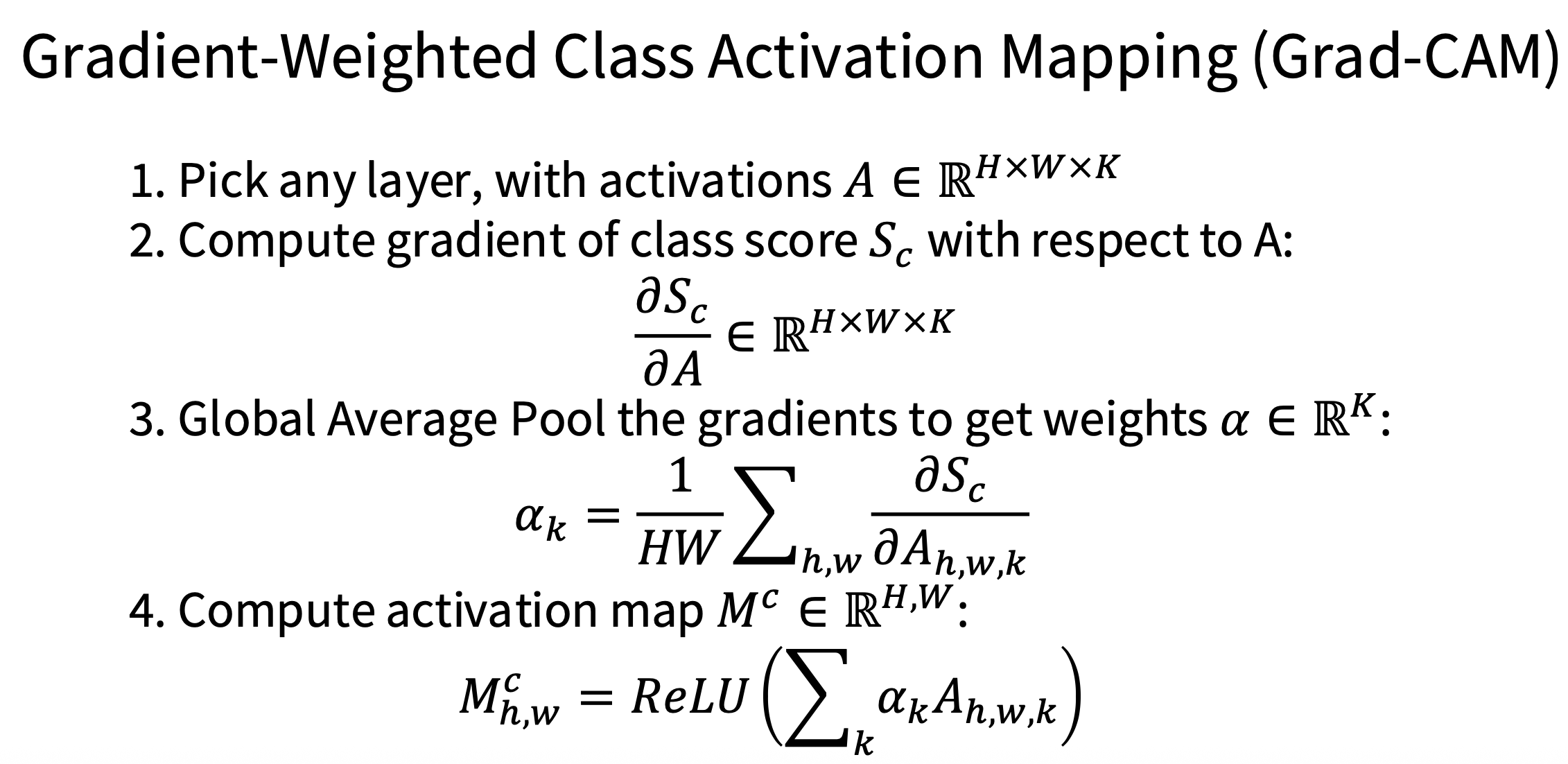
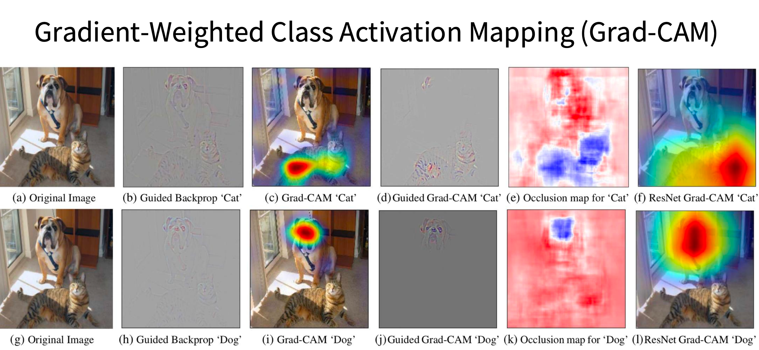
Gradient-Weighted Class Activation Mapping (Grad-CAM)(CVPR 2017)

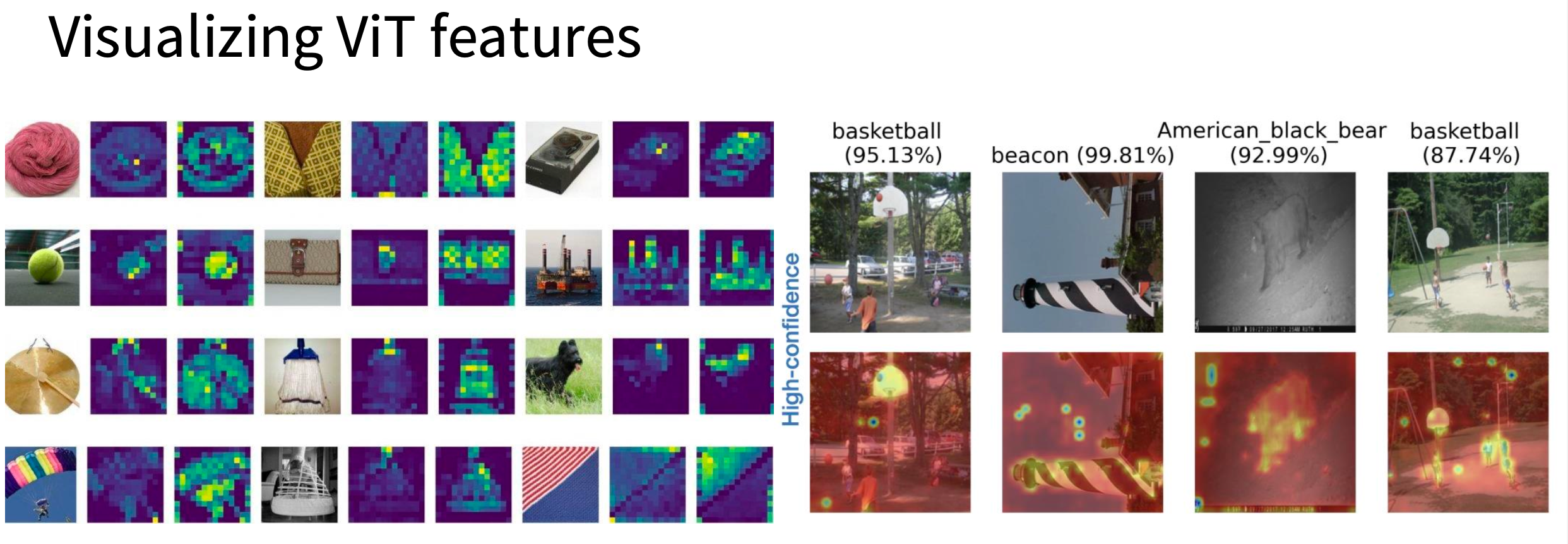
Visualizing ViT features